

How To Set Alerts On Excel Spreadsheet
Tin Excel send Alerts? Aye, only with some limitations. Excel cannot email an alert to y'all automatically unless yous write a macro in the Visual Basic (VBA) editor to perform this part. And, the reminder Alert but works if the Excel software is open. Not quite the convenient method you were hoping for, right?
Another pick, although complicated and limited (at this time) to the XLS spreadsheet formats only, is to set up your spreadsheet similar an Outlook Calendar, then import the data from one to the other. Only this method is not actually a satisfactory result either. And so, until Microsoft decides to provide a functioning solution, we take to settle for work-arounds, using macros plus a petty manual intervention for the email.
Nosotros've created two example spreadsheets for you to use while practicing these tasks:
The example spreadsheet in full, including macros:
Utilise this spreadsheet to practice creating Excel alerts and writing macros for them. Notation: This spreadsheet includes the macros. JD Sartain
The example spreadsheet without the macros, in case y'all're unable to download the i with the macros.
Utilize this spreadsheet to practice creating Excel alerts and writing macros for them. Note: This spreadsheet does NOT include the macros. JD Sartain
Create the spreadsheet, and enter the formulas
You lot tin can setup your spreadsheet to alert you when a borderline is budgeted or when the invoice is due using the Conditional Formatting feature. Then it can send an email to remind you that the invoice is due.
1. Download the Excel Alerts spreadsheet above (without macros) or create or use one of your ain.
2. In cell A1, enter the part: =TODAY().
3. If you're building a spreadsheet from ground zero, enter the post-obit field names in columns A, B, D, and E: Invoices/Debts, Amount Due, Due Twenty-four hours of the Calendar month, Alert Key #, and Alarm Ordinal # on row 4. For column C, type Due Day, press Alt+ Enter (to add a second line), so type of the Calendar month. Practice the same for the stacked headers in the Alert columns E and F.
4. Highlight both columns C and D, then selectHome > Merge & Heart > Merge & Center (from the Alignment group). Middle the remaining field names in columns A, B, E, and F.
v. Populate the database/spreadsheet with some data that matches the fields/column headers.
Because we do non want to create a carve up spreadsheet for every calendar month of the year, we can employ Excel functions to friction match the days of the month to the =TODAY() role, which enters the electric current appointment in prison cell A1 for every single day, 365 days a yr. Merely, unfortunately, twenty-four hour period 10 (or the 10 thursday day of the month) does not match the current engagement; for example; Feb 27, 2022 does not = 27 or 27th. So, we'll employ functions to make them compatible.
6. Enter the function =Twenty-four hours(1) in prison cell C5; =Solar day(2) in C6; =DAY(3) in C7; and so forth down to C34 (for 30 days). (You may enter 31 days if yous similar, but nigh bills are not due on the 31st because that day is not available in every calendar month.)
7. Next, in prison cell A2 enter the part =DAY(A1).
eight. If you prefer ordinal numbers (1st, 2nd, 3 rd, etc.), you can enter the fundamental numbers (one, 2, 3, four, 5) in C5:C34, and so add together this formula in cell D5: =DAY(C5)&IF(OR(Twenty-four hours(C5)={one,2,three,21,22,23,31}),Choose(1*Right(Twenty-four hours(C5),1),"st","nd ","rd "),"th").
9. Copy the formula from D5 downwards through D34 (D5:D34).
10. Add this aforementioned formula to prison cell B2 (merely re-create information technology from D5 to B2, and Excel adjusts the formula to compensate for the new location).
The DAY() function converts the =TODAY() date to a number (due east.g., one, 2, three), which corresponds with ane of the 30 days in whatsoever month. So, regardless of what month the TODAY() part displays, A2 displays only the 24-hour interval.
eleven. Now we need the Alert formulas for columns E and F. Enter this formula in cell E5: =IF(C5=$A$two,"DUE Now", 0). Use Function cardinal F4 to add the $ (dollar) sign, which makes A2 an absolute cell reference (that is, when nosotros copy this formula, column C changes as we copy downwardly, but cell A2 remains the same).
12. Copy the formula in E5 down from E6 through E34.
13. If you prefer the Ordinal numbers, copy this formula into cell F5: =IF(D5=$B$2,"DUE NOW", 0), and then copy the formula in F5 downward from F6 through F34.
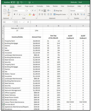 JD Sartain / IDG Worldwide
 Create and populate the spreadsheet, then enter formulas.
Now we tin can create a Conditional Formatting Rule to identify the bills that are due at present.
Utilise Conditional Formatting to create Excel Alerts
one. Highlight E5:E34, then select HOME > Conditional Formatting > New Rule.
ii. In the New Formatting Dominion dialog box underSelect a Rule Type, cull the second pick on the list:Format But Cells that Contain.
iii. In the Edit the Rule Description box nether Format Only Cells With, choose Specific Text from the kickoff field'due south drib-down list, Containing from the second field'south drop-down list, and then enter the words DUE Now in all caps in the third field box.
four. Next, click the Format push button abreast the Preview box.
v. The Format Cells dialog opens. In the Underline field box, choose None course the drop-down list.
half dozen. Under Furnishings, ensure that none of the boxes are checked or blacked-out.
7. Click the pointer abreast the Automatic field box and choose a colour from the palette (e.thou., Red). Notice that the field box name changes from Automatic to Color.
8. In the Font Manner box higher up the Automatic/Color box, select Bold, and so click OK and you did it!
Look down column E Alert Primal # for today's appointment (in this case, February 27th, row 31): The words DUE NOW appear in cell E31, in assuming cerise. Tomorrow, the DUE NOW words will appear on row 32, which corresponds with tomorrow's appointment of Feb 28th.
NOTE: If you lot prefer to piece of work with the Ordinal numbers, follow the instructions above, exactly, except employ the Alerts Ordinal # columns, that is column F, which means the range will be F5:F34.
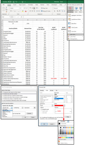 JD Sartain / IDG Worldwide
 Apply Conditional Formatting to create your Alerts
Hmmm, that works great if you don't listen waiting until the very final due appointment to pay your bills. Let'southward create a formula that gives us a few days' notice.
This addition to your spreadsheet is incredibly simple. In jail cell A1, y'all have the formula =TODAY() and Excel returns today's engagement. Press Function central F2 to edit jail cell A1 and add +4 to the end of your formula; that is: =TODAY()+4.
Observe that Excel KNOWS that Feb 27thursday plus 4 equals March 3 rd, fifty-fifty though nosotros're only working with solar day numbers and not days of the month. Otherwise 27 + 4 would equal 31. Pretty smart program, huh? So, at present you have four days' observe before your DUE At present bills are really due.
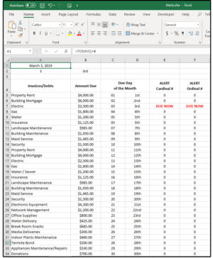 JD Sartain / IDG Worldwide
 Modify ane formula for a four-day notice on bills due.
Prep & electronic mail the spreadsheet
Every bit I mentioned previously, this is not automatic. Y'all could write a macro to do this, but you lot would nevertheless have to open up Excel to run the macro.
If you want to use a macro, which is a bit faster than manually performing these steps, follow the instructions below.
Note: Before you begin the macro, decide whether you want to apply column Due east Cardinal Numbers or column F Ordinal Numbers. Delete the column y'all decide not to use. Discover that the keystrokes are printed in Bold and the comments are in (parentheses).
Turn the Macro Recorder on
1. Click the Programmer tab, then click the Record Macro push button
2. Under Macro Name, type Alerts.
3. Under Shortcut Key, type Shift- Yard. Excel adds the Ctrl key, so the actual macro shortcut keys are Ctrl+ Shift- G.
Note: This is a simultaneous keystroke, which means yous press the Ctrl cardinal and hold, press the Shift key and concur, so press the letter Thou, and release all three keys simultaneously.
4. Under Store Macro In, choose This Workbook (from the list).
5. Under Description enter this text: Located the DUE NOW neb and moves the creditor and amount owed to the top of the spreadsheet.
6. Click OK.
Prep the spreadsheet
Begin recording the post-obit keystrokes (carefully):
1. Printing Ctrl+ Habitation
2. Right, Right, Correct, Right (to delete column Eastward)
or…
3. Right, Right, Right, Correct, Right (to delete cavalcade F)
Notation: Practice not delete both the E and F columns, just one or the other.
4. Click the Domicile tab.
v. Click Delete (in the Cells group).
6. Click Delete Sheet Column (from the driblet-down list).
seven. Ctrl+ Dwelling
eight. Ctrl+ F (The cursor automatically defaults to the Find What field box. Type the search discussion in this box.)
9. Enter: DUE NOW (in all caps).
x. Click the Options button.
11. Click the Look In field box and cull Values from the list.
12. Click the Find Next button.
xiii. Click the Close button.
14. Left, Left, Left, Left
fifteen. Hold down the Shift central and press Correct (one fourth dimension).
xvi. Ctrl+ C
17. Ctrl+ Abode, Right (one time).
eighteen. Ctrl+ V
19. Click the Domicile tab, and choose the Font grouping.
20. Click Font Colour Blood-red, then click Bold.
21. Ctrl+ Home
Now A1 displays today's appointment (plus 4), B1 displays the creditor, and C1 displays the corporeality y'all owe. Information technology doesn't seem similar much of a do good if you lot simply have 30 or so records/rows showing on a single screen, merely if you have 500 records/rows, it's nice to have the nib that's due popular up at the top of the spreadsheet on row ane.
NOTE: If you practise non have the Email push on your Ribbon menu, click File > Options> Customize Ribbon, and add the Email button to the View tab. Read my story on customizing the Give-and-take Ribbon bill of fare for more than information (it works the same in Excel as it does in Word).Practice not finish in the middle of the macro to do the in a higher place procedure. Add the button first, then get dorsum and record the macro.
Email the DUE Now spreadsheet with a message
The following instructions are part of the higher up macro; however, the macro pauses while you lot're in Outlook.
22. Click the View tab.
23. Click the Email button.
Excel opens Microsoft Outlook with a New Email displayed on the screen.
24. The cursor is in the To field; enter the recipient's email address hither.
25. Enter additional email addresses in the CC: field for anyone who should receive a re-create of this email.
Notice that the Alerts spreadsheet is already attached, and the name of the zipper spreadsheet, Alerts.xlsx, is in the subject line.
26. Position the cursor in the trunk of the email and enter the following:
Electric Beak: $2500.00 due March 3
NOTE: Don't bother Copying cells A1:C1 so you can paste them in Outlook. Information technology won't work. One time you enter Outlook, the macro pauses. Everything you lot do in Outlook must be re-keyed every fourth dimension. And, y'all cannot return to Excel until after the open email is sent or cancelled.
27. Click the Send Email button.
Outlook closes and returns yous and your cursor to Excel.
28. Click the Developer tab > Stop Macro button.
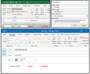 JD Sartain / IDG Worldwide
 Tape the macro and e-mail the spreadsheet.
Exam your macro
1. Printing Ctrl+ Shift- Thousand. (Press the Ctrl central and hold, printing the Shift cardinal and hold, press the letter M, then release all three keys simultaneously.)
2. The macro runs in a second, then opens Outlook for you to enter the email data.
3. And, over again, after you click Send, you're returned to the open up Excel spreadsheet.
Save the spreadsheet as a macro spreadsheet, such asAlerts.xlsm, and exit.
Source: https://www.pcworld.com/article/403377/create-excel-alerts-then-write-a-macro-to-email-them.html
0 Response to "How To Set Alerts On Excel Spreadsheet"
Post a Comment